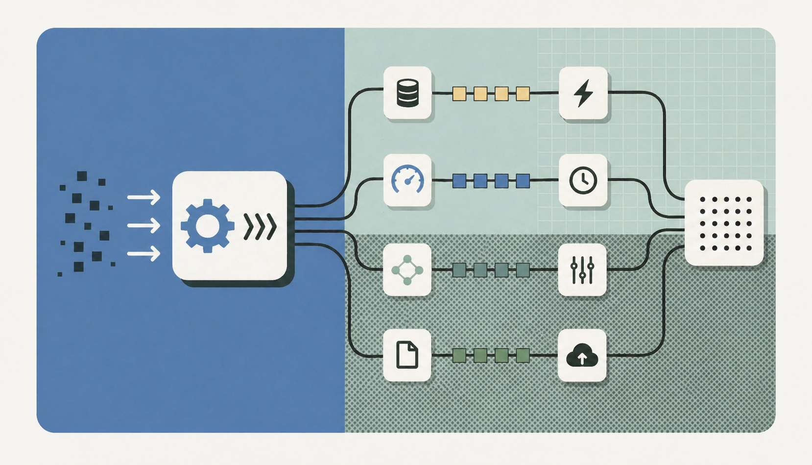
Training ML models requires constructing large datasets by fetching historical features for each loan sample. At Branch’s scale, these training datasets can exceed 1 million samples, making feature fetching one of the slowest parts of the pipeline. We rebuilt our existing pipeline from a single-process serial system into a distributed, actor-based architecture using Ray, cutting the time taken by 8 times with the same resources. This post covers what was slow, why, and the specific optimizations that fixed it.
The 72-Hour Bottleneck
Fetching features for one million loan samples used in training took up to 72 hours in the existing system. Each user requires around 60 different feature families. A feature family is a group of related features computed from the same data source, such as all features derived from a user’s transaction history. Each family contains a median of 60 features, totaling 50 million feature family fetches and 3 billion individual features per run. This slowed down our ability to train models and run experiments at scale.
The bottleneck was the sequential architecture, which had four components:
- A
RecordsIteratorthat reads a parquet file of loan samples and yields user identifiers. - A DynamoDB Fetcher that retrieves cached features for each user.
- A Feature Service Fetcher that computes a user’s features on demand from their historical data.
- A File Writer that flushes the computed features to disk, all running serially in a single process.
The DynamoDB Fetcher and Feature Service Fetcher sat idle while the File Writer wrote to disk, and vice versa. We redesigned this as a distributed, actor-based pipeline using Ray, running all components in parallel alongside several other optimizations, cutting the 1M sample run from 72 hours to ~8 hours with the same resource constraints.
Architecture: From Serial to Parallel Pipeline
The fundamental shift was moving from a single-process loop to an actor-based producer-consumer pipeline. Instead of running all four components sequentially, we split them into independent Ray actors: separate, fault-tolerant processes that communicate through queues. Ray actors are stateful Python classes that run as isolated processes across a cluster. You can learn more in Ray’s actor documentation.
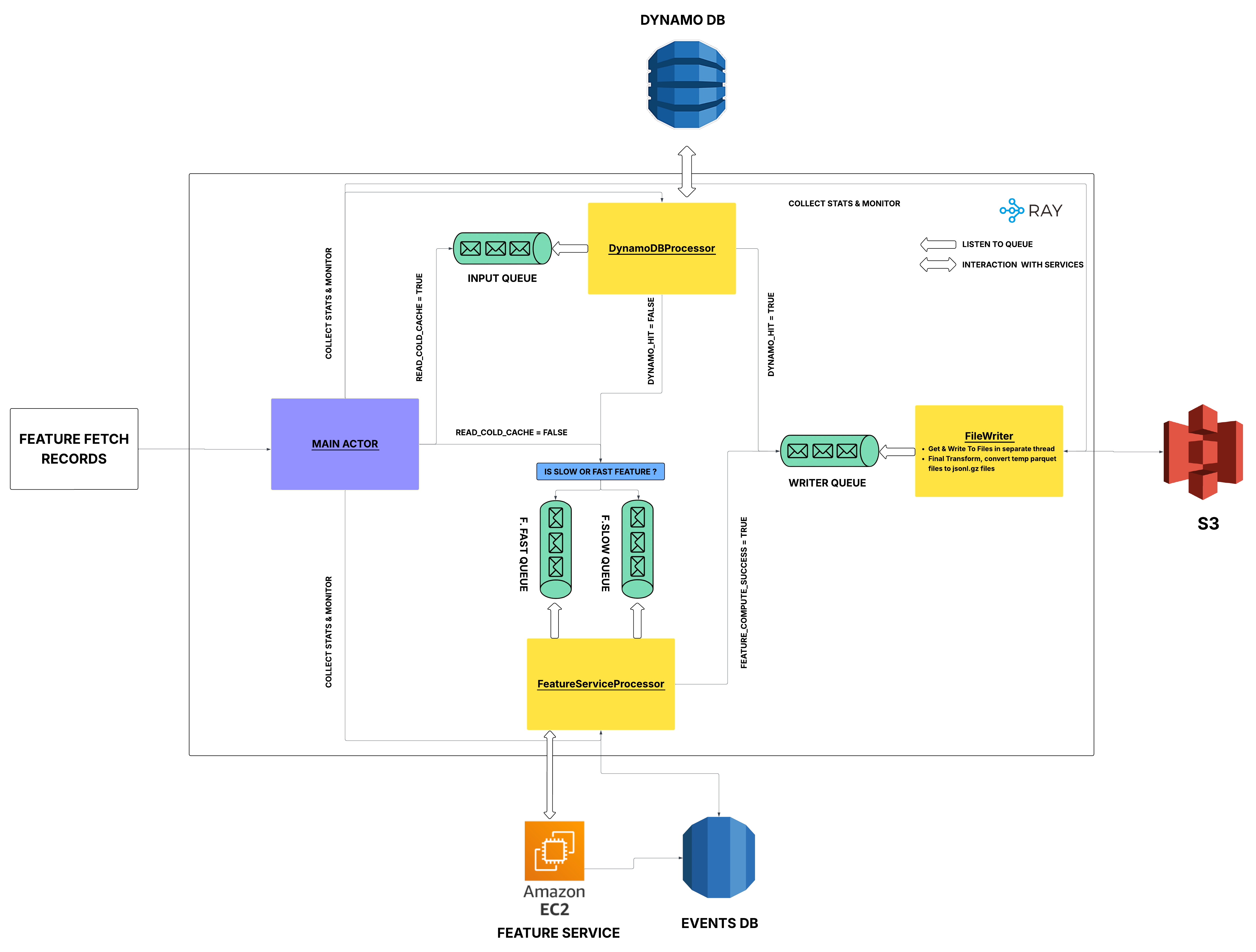
The system has four actors and four queues:
Actors:
- Main Actor: The orchestrator. It spawns worker actors, manages configuration, collects metrics, supervises failures, and coordinates graceful shutdown. Operators interact only with this actor.
- DynamoDB Processor Actor: Listens to the input queue and fetches features from AWS DynamoDB. Cache hits go directly to the Writer Queue. Misses are routed to the Feature Service.
- Feature Service Processor Actor: Listens to the fast and slow feature service queues and fetches features concurrently.
- File Writer Actor: Consumes events from the Writer Queue, writes buffers to Parquet files, performs intelligent batching, and handles the final data transform.
Queues:
- Input Queue: Feature fetch requests waiting to be fetched from AWS DynamoDB.
- Feature Service Fast Queue: All feature families for a user are batched into a single request (1 user → 1 batch request), computed sequentially but fully CPU-intensive.
- Feature Service Slow Queue: Each feature family gets its own parallel request.
- Writer Queue: Successfully fetched features waiting to be written to disk.
Producer-consumer flow:
- The Main Actor reads records and intelligently routes them to the appropriate queue (Input, Feature Service Fast, or Slow), based on the characteristics of each feature family.
- The DynamoDB and Feature Service Processor Actors independently fetch features and puts their results into the Writer Queue.
- The File Writer Actor consumes results from the Writer Queue, buffers them, and flushes to disk once the buffer is full.
- A cache file is updated with completed feature families, enabling incremental recovery and efficient restarts after failure.
- Completed output files are synced to AWS S3 for durability and fault tolerance.
In the old system, all feature families for a user were fetched and written together as one job. In the new Feature Fetch, the atomic unit is a feature family: each family is dispatched, fetched, and written independently as soon as it arrives. This avoids bloating the queue with partial user data, keeps memory usage low, and gives the pipeline flexibility to route slow and fast feature families separately.
Each actor type can be scaled by launching more instances of it as independent Ray processes, each running on its own CPU core and pulling from the same shared queue. Adding actors only increases speed when existing actors are already saturated and the Feature Service, DynamoDB and Databases can handle more load:
- The Main Actor is lightweight, scaling it has no effect.
- The DynamoDB Fetcher is CPU-bound. Scaling it helps, provided DynamoDB has sufficient read capacity.
- The Feature Service Processor is I/O-bound, constrained by the Feature Service and the IOPS available on the RDS.
- The File Writer is constrained by the speed at which DynamoDB and Feature Service Actors process features. It can scale freely since concurrent writes without conflicts are guaranteed through per-actor file ownership, and it yields the most benefit when DynamoDB fetches are fast.
Since these are Python processes bound by the GIL, each actor uses one CPU core. More actors means more processes, means more CPU parallelism.
Configuration: We use a Pydantic config object to define actor counts, queue configs, and all run parameters. The reason to choose Pydantic is that it provides extensive validation for all configuration fields at startup, ensuring invalid values are caught before any fetching begins. The config also serves as a job queue, drawing fetch jobs iteratively from AWS S3 so the system processes continuously as new jobs arrive.
Solving the Fetching Bottlenecks
With the new architecture in place, the more challenging optimizations were figuring out why DynamoDB and Feature Service fetching were slow, and fixing them. These two components work in tandem: AWS DynamoDB serves cached features, and anything it misses gets routed to the Feature Service for on-the-fly computation. Both had their own set of problems.
The DynamoDB Insight: CPU-Bound, Not I/O-Bound
Our legacy code used a default batch size of 100, assuming the AWS DynamoDB fetcher was I/O-bound. Profiling revealed it’s actually CPU-bound: the time spent creating keys and processing batch requests exceeds the time spent fetching from AWS DynamoDB. Even increasing the batch size to 1,000 didn’t help proportionally. A single CPU core won’t see improvements beyond a connection pool size of 3 (with shared connections and async requests). At that optimal pool size, one core tops out at 8,000 requests/second. Rather than pushing pool size higher which still gets executed on a single CPU, we parallelized the load across cores/actors to maximize throughput. Batching requests, shared connections, and async requests on a single core yielded a 3x speedup. Parallelizing across multiple actors multiplies this by the number of cores, giving us n × 3x as long as we stay within our DynamoDB read provisioning limits.
The Feature Service Strategy: Fast vs. Slow Queues
The Feature Service had a different set of problems entirely:
-
Too many requests: The old flow split each user’s feature families into groups of 3 per Feature Service request. This made sense for inference, as minimizing latency for a single user is crucial. But for batch fetching, the goal is minimize the time taken for feature fetch across all users, not low latency for any one user. With approx 60 feature families per user in groups of 3, we sent 20 requests per user, or 20,000 requests for 1,000 users. The Feature Service (36 pods, 6 effective CPUs each, 150 threads each) had CPU utilization hovering around 30% as most cycles went to managing thousands of concurrent requests, not actual computation.
-
Slow feature families blocking fast ones: Different feature families have varying data sizes and computational requirements, which can cause some families to be slower than others. One main example is the event features which reads from an Amazon RDS database with ~100 billion rows, which is completely I/O-bound. Another one is that African market features run heavy regex operations on huge chunk of SMS’es, which is CPU-bound. In the old flow, mixing slow and fast families in the same request meant every request could get stuck. Since the Feature Service uses a synchronous Flask server, multiple slow I/O-bound requests in the same batch execute sequentially, compounding the problem.
-
Synchronous server with no easy workaround: Each request blocks a thread. Moreover, converting the Feature Service to async wouldn’t solve the root problem, it would just shift the bottleneck to the RDS database. That database already runs near its IOPS limit (GP3 storage caps at 64,000 IOPS), and upgrading to faster storage would require significant cost and effort. We had to work with what we had.
The fix: Two queues with semaphore-controlled concurrency. The core insight was that fast and slow feature families have fundamentally different processing profiles and shouldn’t share the same request queue.
- Fast queue: All feature families for a user are batched into one Feature Service request. Features execute sequentially within the request, but efficiently, with no blocking from slow families.
- Slow queue: Each feature family gets its own parallel request, preventing slow families from stalling each other.
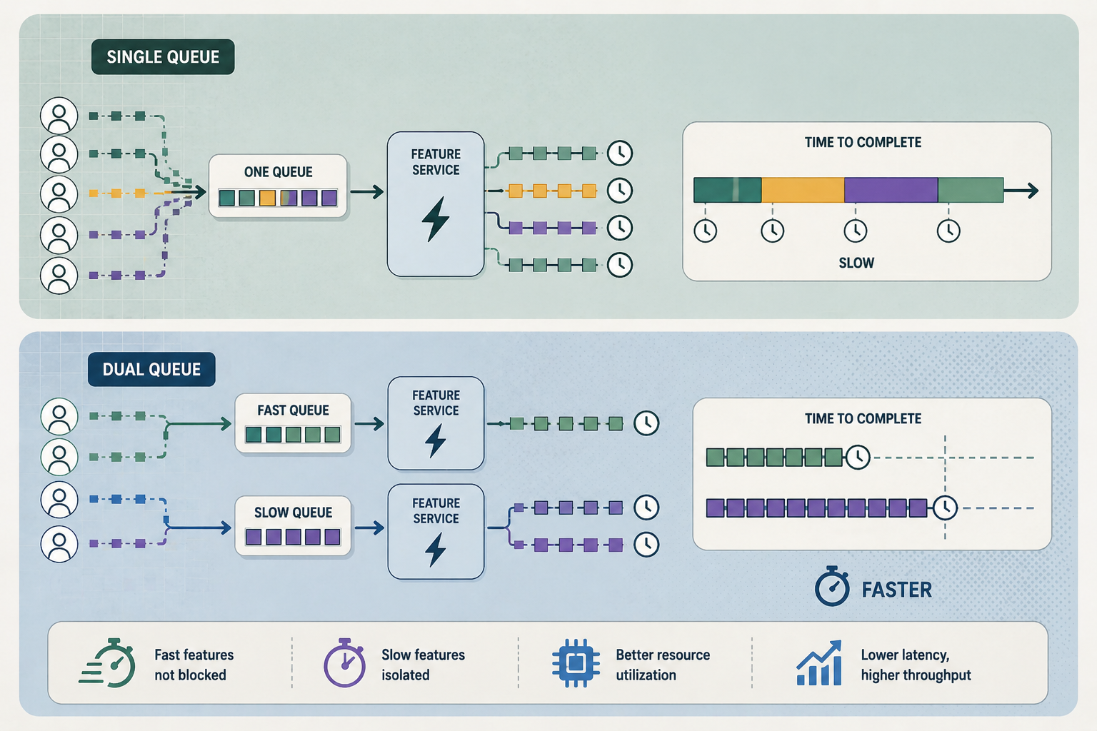
For each user, one fast request handles all the fast families while each slow family runs independently. Both paths are sized to finish around the same time, minimizing the cost of thread switching and I/O wait time without overloading the Feature Service.
Why not a single queue? When we send all requests as one combined flow, they accumulate faster than they can be processed, leaving no room to take on new work. The entire system, or most of it, becomes I/O-bound as slow families (large RDS scans) dominate the in-flight slots. Controlling how many I/O-bound requests run at once is what keeps capacity free so other requests can actually get computed. On top of that, a single queue gives no way to split capacity deliberately: giving the top X slowest families Y% of allowed in-flight bandwidth means they can compute without competing for every slot, while the remaining families share the other 100 − Y%. Splitting limits that way is what moves the batch toward a local minimum of total compute time.
Semaphores (Feature Service side). Semaphores sit on the Feature Service side to enforce that bandwidth split: they assign how much concurrency each slice of work gets, keyed by queue/family (e.g. slow_feature_family_pool_size per family name). A semaphore is a counter that blocks at zero: tasks acquire a slot before work and release it when done, so bandwidth is handed out deliberately and the Feature Service can complete computation for the job as a whole more effectively than with one undifferentiated queue.
Connection pooling further eliminates TCP + TLS handshake overhead (10-50ms per request) by sharing one aiohttp.TCPConnector pool across all requests. Connection reuse, DNS caching, TCP keep-alive, and TLS session resumption all compound across thousands of requests, cutting overhead that would otherwise add up to significant time.
The dual queue logic combined with right-sizing the Feature Service workers produced an 8x speedup in this component. Before, we ran 20 workers with 250 threads per pod, had 40,000 requests live at any point in time, and still only hit 40% CPU utilization as most threads were waiting and cpu is switching threads, not computing. After, we dropped to 8 workers and 10 threads per pod (sized for 6 CPUs), with around 1,000 requests live at one time, and CPU utilization reached 100%. Fewer in-flight requests, fully utilized CPUs, and no slow families blocking fast ones is what drove the improvement.
The Writer: Solving Blocking Writes and OOMs
In the old system, writing was straightforward: since every request to DynamoDB and the Feature Service was at the user level, all features for a user arrived together and could be written directly to a jsonl file. The new pipeline changed that. The atomic unit is now a feature family, not a user. Features for the same user arrive from different actors at different times, some from DynamoDB, some from the features service slow pool, some from the feature service fast queue, with no guarantee of ordering. We cannot write a user’s jsonl record until all their feature families have been collected. So we introduced an intermediate storage layer: the writer saves data as it arrives, one record per feature family, in a narrow Parquet format. When a writer accumulates enough records or hits the per-file limit, it flushes to disk.
As we scale DynamoDB and Feature Service actors to increase throughput, the number of writers scales with them. Without a clear ownership model, multiple actors writing to the same file would corrupt data or overwrite each other’s results. Each File Writer Actor writes to its own uniquely named file (actor_id + uuid + file_counter), so every actor owns its own output with no race conditions regardless of how many actors are running.
This introduces a new problem. Our training pipeline requires jsonl.gz files, so Parquet has to be converted back. Rewriting the pipeline to consume Parquet directly would work in theory, but it would introduce significant engineering effort and new bugs across systems that are already in production. Reading all 50M feature family rows at once, grouping them by (user_id, score_timestamp), and pivoting to a wide format is memory intensive, slow, and does not scale beyond a few hundred thousand users. At 1M+ users it causes OOM failures in smaller pods.
The fix: hash-based chunking, and sorting.
At write time, each record is assigned to a chunk using a deterministic hash so that all features for the same (user_id, score_timestamp) always land in the same chunk directory. At final transform time, instead of reading all Parquet files at once, we process one chunk directory at a time. Each directory holds multiple Parquet files written by different actors and different batches. Each folder gets its own independent Ray task that reads only those files, pivots them, and writes a single output shard. Tasks run in parallel, each touching only a fraction of the total data:
-
Chunk assignment (Main Actor): Before starting to process, the Main Actor builds a chunk ID mapping:
chunk_id = hash(user_id, score_timestamp) % num_chunks. The chunk count is dynamic:num_chunks = ceil(total_users / batch_size)(e.g.batch_size=5000gives 4 chunks for 20k users, 200 chunks for 1M users). This mapping is broadcast to all File Writer actors, so every writer uses the same assignment. -
Write phase (File Writer): Writers group records by chunk ID using the shared mapping and write to dedicated directories:
chunk_00000/,chunk_00001/, etc. All features for the same(user_id, score_timestamp)land in the same chunk directory, even when fast and slow features arrive in different writer batches, because the hash is deterministic. However, there is an fundamental problem though: users within a chunk are scattered across the original sample, so as records arrive in processing order, each buffer contains feature families from many different chunks. This meant the writer had to flush a separate file for each batch, producing around 15,000 small files for 1M users. Each small file is an IOPS cost that slows the writer down. The fix to this was to sort the input records by chunk ID on the Main Actor before dispatching them. This groups all feature families belonging to the same chunk together in the stream, so a writer buffer is far more likely to be filled entirely by one chunk before flushing. That reduced file writes from 15,000 down to around 1,000 for 1M users, significantly speeding up the writer. -
Final transform (one task per chunk): As mentioned above, instead of reading all Parquet files at once, final transform lists chunk directories and runs one Ray task per chunk in parallel. Each task reads only the Parquet files in that chunk’s directory, pivots to wide format, and writes a single shard (e.g.
chunk_00000.jsonl.gz). After all shards are written, temporary chunk directories are removed locally and on AWS S3.
Why this works:
- Memory: Peak memory drops significantly, with many tasks running in parallel across the cluster. OOM risk for 1M+ users is effectively removed.
- Parallelism: Final transform is no longer single-threaded. One chunk equals one Ray task, so it scales with available CPUs (e.g. 200 chunks gives up to 200 concurrent tasks).
- Correctness: The same
(user_id, score_timestamp)always maps to the same chunk, so fast and slow features for the same user are merged correctly when the chunk is pivoted. - Scalability: Chunk count grows with dataset size (
batch_sizecontrols users per chunk), so small runs don’t create too many chunks and large runs get enough parallelism without manual tuning.
Operational Excellence: Warm-up, Caching, and Graceful Shutdown
A fast pipeline that leaves resources over-provisioned or crashes without cleanup isn’t production-ready. We handle the full lifecycle explicitly:
-
Warm-up: Before fetching starts, the system scales up AWS DynamoDB read/write capacity, Feature Service pods, and the RDS instance in parallel, all sized by the configuration object. Once all services are ready, the fetch begins.
-
Incremental caching and fault recovery: After each buffer is flushed, the writer updates a cache file keyed by
(user_id, score_timestamp, feature_family_id). On the next run, the Main Actor reads this cache at startup and skips any feature family that was already successfully written. If the job fails or is interrupted mid-run, restarting it picks up exactly where it left off without re-fetching or re-writing completed work. This makes long runs resilient to transient failures without any manual intervention. -
Retry logic and monitoring: The Main Actor monitors each worker continuously. On failures, it applies per-family retry logic: transient errors on a specific feature family trigger a targeted retry for that family rather than restarting the entire job. Some families are known to be flaky under load (event features hitting RDS limits), so retry budgets and backoff strategies are configured per family. For persistent failures across families or signs of a wider outage (service unavailability, database errors, repeated schema mismatches), the Main Actor decides whether to restart the affected actor or shut the system down cleanly. This fine-grained monitoring and retry logic improved overall stability significantly, reducing the number of full job failures in production.
-
Graceful shutdown: The Main Actor registers shutdown handlers at startup to ensure provisioned resources are always scaled back down, regardless of how the process exits: normal completion, exception, Ctrl+C, or SIGTERM. No over-provisioned resources left behind, regardless of how the run ends.
Impact and Results
Through careful analysis and architectural redesign, we built Fast Feature Fetch, a distributed, parallel actor-based system. Here’s what changed:
| Area | Before | After | Improvement |
|---|---|---|---|
| Run time (1M samples) | 72 hours | ~8 hours | 8× faster |
| Feature Service CPU utilization | ~40% | 100% | Increased resource efficiency[1] |
| Feature Service requests | ~40,000 in-flight | ~1,000 in-flight | 90% reduction |
| Feature Service workers / threads | 20 workers, 250 threads | 8 workers, 10 threads | Right-sized for 6 CPUs |
| DynamoDB throughput | Baseline | 3× per core, n× across actors | 6× overall speedup |
| Max analysis scale | ~300K samples/day | 5M samples/day | Limitlessly scalable |
[1] 100% CPU utilization and 70% lower memory usage let us move to compute-optimized instances with more CPUs per pod at lower cost.
Disclaimer: All personally identifiable information (PII) used in the experiments described in this post was anonymised before analysis. No raw PII is included in the results, examples, or diagrams shared here.
Comments
Loading comments…